Interpolating with brille
In this tutorial you will interpolate two things with brille: a linear field, which linear interpolation reproduces exactly, and the spin-wave dispersion of iron, which it approximates. Along the way you will meet the three objects every brille interpolation needs: a lattice, its Brillouin zone, and a grid.
The code is one script, interpolation.py, which the tests
run. You need brille and NumPy, and matplotlib for the plots.
A linear field
The lattice
A grid spans part of reciprocal space, so start with a lattice. This one is given directly in reciprocal space: three orthogonal basis vectors, each 1 Å⁻¹ long.
from brille import Lattice

lattice = Lattice(((1, 1, 1), (90, 90, 90)), real_space=False)
print(f"reciprocal cell volume {lattice.volume_star:.3f} Å⁻³")
The Brillouin zone
A grid's extent is always a first or irreducible Brillouin zone, which
BrillouinZone finds from the lattice:
from brille import BrillouinZone

zone = BrillouinZone(lattice)
print(f"first zone {zone.polyhedron.volume:.3f} Å⁻³, irreducible zone {zone.ir_polyhedron.volume:.3f} Å⁻³")
first zone 1.000 Å⁻³, irreducible zone 1.000 Å⁻³
The lattice was given no symmetry, so it has only the identity operation, and its irreducible zone is the whole first zone: the cube from −½ to ½ along each axis.
The grid
BZMeshQdd is a mesh of tetrahedra that fills the
irreducible zone and holds real (d, for double) data. max_size bounds the
volume of its tetrahedra, in Å⁻³, which sets how many points it has:
from brille import BZMeshQdd

grid = BZMeshQdd(zone, max_size=zone.ir_polyhedron.volume / 100)
print(f"{len(grid.rlu)} grid points")
Its points are grid.rlu, in reciprocal lattice units, and grid.invA, in
Å⁻¹; for this lattice the two are the same.
Fill the grid
A grid holds values (scalars, such as energies) and vectors (such as
eigenvectors) at each point, and fill
takes both, with a description of each. Here each point holds one scalar,
\(\phi(\mathbf{Q}) = \mathbf{Q}\cdot\hat{\mathbf{x}}\), given as both values and
vectors:
def phi(q):
    """A linear scalar field, the first Cartesian component of q"""
    return np.asarray(q)[:, 0]


values = phi(grid.invA)[:, np.newaxis]   # one value per grid point
elements = (1,)                          # each point holds one scalar
grid.fill(values, elements, values, elements)
Interpolate
ir_interpolate_at returns the
interpolated values and vectors at any points. Inside the zone, linear
interpolation of a linear field is exact:
q = np.random.default_rng(1).random((10, 3)) - 0.5   # inside the first zone
interpolated, _ = grid.ir_interpolate_at(q)
print(f"inside the zone, exact: {np.allclose(interpolated[:, 0], phi(q))}")
A point outside the zone is first moved into it by a reciprocal lattice vector \(\mathbf{G}\), so the result there is \(\phi(\mathbf{Q}-\mathbf{G})\), not \(\phi(\mathbf{Q})\): brille assumes the data are periodic in the reciprocal lattice, as physical properties of a crystal are.
far = 20 * q                                          # anywhere in (-10, 10)
interpolated, _ = grid.ir_interpolate_at(far)
print(f"outside the zone, phi(Q - G): {np.allclose(interpolated[:, 0], phi(far - np.round(far)))}")
inside the zone, exact: True
outside the zone, phi(Q - G): True
Iron's spin waves
A dispersing excitation has an energy that depends on \(\mathbf{Q}\). Iron's acoustic ferromagnetic spin wave has
with \(Q_i\) in reciprocal lattice units, a single-ion anisotropy \(\delta\) and an exchange energy \(J\). It has the periodicity and symmetry of iron's lattice, so brille can interpolate it.
The lattice and grid
Iron is body-centred cubic, \(a = 2.87\) Å, with space group \(Im\bar{3}m\). Its 48 point symmetry operations make the irreducible zone a forty-eighth of the first zone, and the grid needs to cover only that:
iron = Lattice(((2.87, 2.87, 2.87), (90, 90, 90)), spacegroup="Im-3m")
iron_zone = BrillouinZone(iron)
iron_grid = BZMeshQdd(iron_zone, max_size=iron_zone.ir_polyhedron.volume / 6000)
print(f"iron: irreducible zone {iron_zone.ir_polyhedron.volume / iron_zone.polyhedron.volume:.4f} "
      f"of the first, {len(iron_grid.rlu)} grid points")
iron: irreducible zone 0.0208 of the first, 1741 grid points
Fill and check
def omega(q, exchange=16, anisotropy=0.01):
    """Iron's acoustic spin-wave energy, in meV, at q in reciprocal lattice units"""
    return anisotropy + 8 * exchange * (1 - np.prod(np.cos(np.pi * np.asarray(q)), axis=1))


energies = omega(iron_grid.rlu)[:, np.newaxis]
iron_grid.fill(energies, elements, energies, elements)
At its own points, the grid returns exactly what it was given:
at_vertices, _ = iron_grid.ir_interpolate_at(iron_grid.rlu)
print(f"the grid returns its own values: {np.allclose(at_vertices, energies)}")
Interpolate along a path
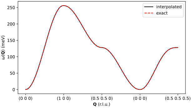
Between its points, the grid interpolates linearly, so it differs from the curved dispersion. Along a path through the zone, from Γ to H \((1\,0\,0)\), N \((\tfrac12\,\tfrac12\,0)\), back to Γ and on to P \((\tfrac12\,\tfrac12\,\tfrac12)\):
corners = np.array([[0, 0, 0], [1, 0, 0], [0.5, 0.5, 0], [0, 0, 0], [0.5, 0.5, 0.5]])
per_leg = 100
path = np.vstack([np.linspace(corners[i], corners[i + 1], per_leg) for i in range(len(corners) - 1)])
along, _ = iron_grid.ir_interpolate_at(path)
error = np.abs(along[:, 0] - omega(path))
print(f"along the path: largest error {error.max():.2f} meV of {omega(path).max():.0f} meV")
along the path: largest error 0.45 meV of 256 meV
Most of the path lies outside the irreducible zone. ir_interpolate_at
maps each point into it with a symmetry operation and a lattice vector.
import matplotlib.pyplot as plt

x = np.arange(len(path))
ticks = [*(per_leg * np.arange(len(corners) - 1)), len(path) - 1]
labels = ["(" + " ".join(f"{c:g}" for c in corner) + ")" for corner in corners]

def plot(ax):
    ax.plot(x, along[:, 0], "-k", label="interpolated")
    ax.plot(x, omega(path), "--r", label="exact")
    ax.set_xticks(ticks, labels)
    ax.set_xlabel(r"$\mathbf{Q}$ (r.l.u.)")
    ax.set_ylabel(r"$\omega(\mathbf{Q})$ (meV)")

fig, ax = plt.subplots(figsize=(6.4, 3.6), layout="constrained")
plot(ax)
ax.legend()
Close to the maximum at H, the straight segments of the interpolation are visible:
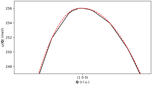
A finer grid, a smaller max_size, reduces the error.
Building and refining a mesh shows how to add points only where
they are needed.